Perform Linear Regression in Azure Databricks with MLLib

When thinking of performing machine learning, especially in Python, a few frameworks may come to mind such as scikit-learn, Tensorflow, and PyTorch. However, if you're already doing your big data processing in Spark, then it actually comes with its own machine learning framework - MLLib.

In this post, we'll go over using MLLib to create a regression model within Azure Databricks. The data we'll be using is the Computer Hardware dataset from the UCI Machine Learning Repository. The data will be on an Azure Blob storage container, so we'll need to fetch the data from there to work with it.

What we would want to predict from this data is the published performance of the machine based off of its features. There is a second performance column at the end, but looking at the data description that is what the original authors predicted using their algorithm. We can safely ignore that column.

If you would prefer a video version of this post, check below.

Connecting to Azure Storage

Within a new notebook, we can set some variables, such as the storage account name and what container the data is in. We can also get the storage account key from the Secrets utility method.

storage_account_name = "databricksdemostorage"
storage_account_key = dbutils.secrets.get("Keys", "Storage")
container = "data"

After that we can set a Spark config setting specifically within Azure Databricks that can connect the Spark APIs to our storage container.

spark.conf.set(f"fs.azure.account.key.{storage_account_name}.blob.core.windows.net", storage_account_key)

For more details on connecting to Azure Storage from Azure Databricks, check out this video.

Using the APIs we can use the read property on the spark variable (which is the SparkSession) and set some options such as telling it to automatically infer the schema and what the delimiter is. Then the csv method is called with the Windows Azure Storage Blob URL (WASB), which is built on top of HDFS. With the data fetched we then call the show method on it.

However, looking at the data, it defaults the column names. Since we'll be referencing the columns, it'll be nice to have names to them to make referencing them easier. To do this we can create our own schema and use that when reading the data.

To read the schema we'll need to create it using StructType and StructField which help specify a schema for a Spark DataFrame. Don't forget to import these from pyspark.sql.types.

from pyspark.sql.types import StructType, StructField, StringType, DoubleType

schema = StructType([
  StructField("Vendor", StringType(), True),
  StructField("Model", StringType(), True),
  StructField("CycleTime", DoubleType(), True),
  StructField("MinMainMemory", DoubleType(), True),
  StructField("MaxMainMemory", DoubleType(), True),
  StructField("Cache", DoubleType(), True),
  StructField("MinChannels", DoubleType(), True),
  StructField("MaxChannels", DoubleType(), True),
  StructField("PublishedPerf", DoubleType(), True),
  StructField("RelativePerf", DoubleType(), True)
])

With this schema set we can pass that into the read property with the schema method and pass this in as the parameter. Since we pass in the schema we no longer need the inferSchema option. Also, we can now tell Spark to use a header row.

data = spark.read.option("header", "true").option("delimeter", ",").schema(schema)
  .csv(f"wasbs://.blob.core.windows.net/machine.data")

data.show()

Splitting the Data

With our data now set, we can start building our linear regression machine learning model with it. The first thing to do, though, is to split our data into a training and testing set. We can do this with the randomSplit method on the Spark DataFrame.

(train_data, test_data) = data.randomSplit([0.8, 0.2])

The randomSplit method takes in a list as a parameter and the first item of the list is how much to keep in the training set and the second item is how much to take in the testing set. This returns a tuple which is why there are parentheses around the variables.

Just because I'm curious, let's see what the count of each of these dataframes are.

print(train_data.count())
print(test_data.count())

Creating Linear Regression Model

Before we can go further, we need to make some additional imports. We need to import the LinearRegression class, a class to help us vectorize our features, and a class that can help us evaluate our model based on the test data.

from pyspark.ml.regression import LinearRegression
from pyspark.ml.feature import VectorAssembler
from pyspark.ml.evaluation import RegressionEvaluator

Now, we can begin building our machine learning model. The first thing we need is to create a "features" column. This column will be an array of all of our numerical columns. This is what the VectorAssembler class can do for us.

vectors = VectorAssembler(inputCols=['CycleTime', 'MinMainMemory', 'MaxMainMemory', 'Cache', 'MinChannels', 'MaxChannels'], outputCol="features")

vector_data = vectors.transform(train_data)

For the VectorAssembler we give it a list of input columns that we want to vectorize into a single column. There's also an output column parameter in which we specify what we want the name of the new column to be.

NOTE: To keep this simple, I'll exclude the text columns. Don't worry, though, we'll go over how to handle this in a future post/video.

We can call the show method on the vector data to see how that looks.

vector_data.show()

Notice the "features" column was appended on to the DataFrame. Also, you can tell that the values match each value in the other columns in that row. For instance, the first value in the "features" column is 29 and the first value in the "CycleTime" column is 29.

Let's clean up the DataFrame a bit and only have the columns we care about, the "features" and "RelativePerf" columns. We can do that just by using the select method.

features_data = vector_data.select(["features", "PublishedPerf"])

features_data.show()

With our data now updated to the format the algorithm wants, let's actually create the model. This is where we use the LinearRegression class from the import.

lr = LinearRegression(labelCol="PublishedPerf", featuresCol="features")

With that class we give it a couple of parameters in the constructor, what the label column name is and what the name of the features column is.

Now we can fit the model based on our data.

model = lr.fit(features_data)

And now we have our model! We can look into it by getting the model summary and examining the R Squared on it.

summary = model.summary

print("R^2", summary.r2

From here, it looks like it performs quite well with an R Squared of around 91%. But let's evaluate the model on the test data set. This is where we use the RegressionEvaluator class we imported.

evaluator = RegressionEvaluator(predictionCol="prediction", labelCol="PublishedPerf", metricName="r2")

This takes in a few constructor parameters which include the label column name, the metric name we want to use for our evaluation, and the prediction column. The prediction column we'll get when we when we run the model on our test set.

With our evaluator defined, we can now start to pass data to it. But first, we actually need to make our test dataset into the same format that we did our training data set. So we'll need to follow the same steps to vectorize our data.

vector_test = vectors.transform(test_data)

Then, select the columns we care about using.

features_test = vector_test.select(["features", "PublishedPerf"])

Now we can use the model to make predictions on our test data set and we'll show those results.

test_transform = model.transform(features_test)

test_transform.show()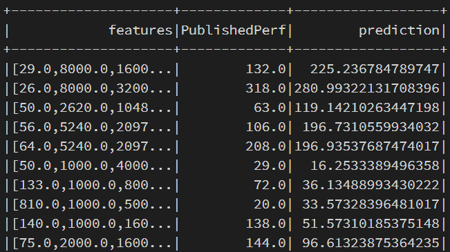

The prediction column are the predicted values. You can do a bit of a comparison to that and the "PublishedPerf" column. Do you think this model will perform well based on what you see?

With the predictions on the test dataset we can now evaluate our model based on that data.

evaluator.evaluate(test_transform)

Looks like the model doesn't perform very well with this R Squared being 56%, so there is probably some feature engineering we can do.

If you watched the video and saw that the evaluation returned 90%, then it's possible the split got different data that caused this discrepancy. This is a good reason to run cross validation on your data.

---

Hopefully, you've learned some things with this post about using MLLib in Azure Databricks. Things to take away is that MLLib is built into Spark and, therefore, built into Azure Databricks so there's no need to install another library to perform machine learning on your data.

A Quick Tour of Azure Databricks

I did a webinar a while back on Azure Databricks. Below is an section of the webinar that goes over how to create an instance of it and shows some of the UI of Databricks. Hope you enjoy!

And if you're interested in seeing the entire webinar, here it is below.

How to Read Azure Data Lake Storage in Azure Databricks

When trying to read files in Azure Data Lake storage in Azure Databricks is definitely possible, doing so takes quite a few steps. In this video, I show those steps exactly. Hope this helps make it easier for you to connect from data lake storage to Databricks.